Microreactor Mixing and Residence Time Distribution for Design and Scale-Up

Microreactor performance depends on two closely related transport characteristics. Mixing determines how quickly reactants become homogenized, while residence time distribution (RTD) describes how long individual fluid elements remain inside the reactor.

These parameters influence conversion, selectivity, heat release, and product consistency. In fast competitive reactions, local concentration gradients can favor undesired reaction pathways even when the average residence time meets the design target. A broad RTD can further expose different fluid elements to different reaction histories.

For process engineers, the design challenge is to quantify both effects and preserve the required transport behavior during scale-up. This requires combining mixing-time correlations, axial dispersion models, tracer-based RTD measurements, and flow distribution analysis.

DODGEN’s تكنولوجيا المفاعلات الصغيرة provides an industrial context for evaluating these relationships in continuous chemical manufacturing.

Why Mixing and Residence Time Distribution Matter in Microreactors

Microreactors provide short transport distances and high surface-area-to-volume ratios, making them suitable for processes requiring rapid heat and mass transfer. However, small channel dimensions do not automatically guarantee uniform mixing or ideal plug flow.

Actual performance depends on channel geometry, fluid properties, molecular diffusivity, flow rate, and reactor configuration. These variables determine the relative contributions of molecular diffusion, convection, and hydrodynamic dispersion.

Ideal Plug Flow and Non-Ideal Flow Behavior

An ideal plug flow reactor (PFR) assumes that fluid elements move through the reactor without axial mixing and experience approximately the same residence time.

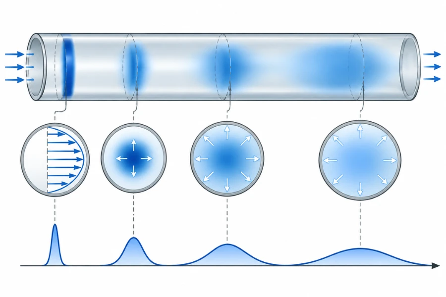
Real microchannels can deviate from this behavior. Under laminar flow, the parabolic velocity profile in a straight circular channel creates different axial velocities across the cross-section. Fluid near the center moves faster than fluid near the walls, producing a distribution of residence times.

Molecular diffusion transfers material between adjacent streamlines, but its ability to reduce this variation depends on the transverse diffusion distance and available residence time.

Inlet and outlet geometry, dead volumes, recirculation zones, surface interactions, and parallel-channel flow maldistribution can further affect the measured RTD.

Mixing Time vs. Mean Residence Time

Mixing time and mean residence time describe different physical processes and should not be used interchangeably.

المعلمة	Mixing Time	Mean Residence Time
التعريف	Time required to reach a specified degree of mixing	Average time fluid elements spend inside the reactor
Main factors	Diffusivity, mixing geometry, velocity, and flow structure	Reactor volume and volumetric flow rate
Engineering purpose	Evaluate mixing limitations	Evaluate reaction contact time
القياس	Concentration homogenization or mixing-sensitive methods	Tracer-based RTD measurement

The nominal space time of a single-phase continuous reactor is:

[\tau=\frac{V}{Q}]

For a uniform channel with cross-sectional area (A), length (L), and average velocity (u):

[\tau=\frac{AL}{Au}=\frac{L}{u}]

This value provides a design reference but does not describe the complete residence time distribution.

A reactor can have a nominal space time of 25 seconds while individual fluid elements experience different residence times. Tracer testing is needed to quantify the actual distribution.

Mixing Mechanisms and Transport Behavior in Microreactors

Mixing in microreactors results from the interaction of molecular diffusion and fluid motion. Because many microchannels operate under laminar conditions, transverse transport and channel geometry are particularly important.

Molecular Diffusion and Convective Mixing

Molecular diffusion transports species from regions of higher concentration toward regions of lower concentration. Its characteristic timescale across a distance (d) can be estimated as:

[t_D\sim\frac{d^2}{D_m}]

Where (D_m) is the molecular diffusion coefficient.

Halving the diffusion distance reduces the characteristic diffusion time by approximately a factor of four, assuming the same diffusivity. This explains why reducing the distance between reactant streams can be more effective than simply increasing reactor volume.

Convective mixing uses fluid motion to redistribute material. Split-and-recombine structures, curved channels, grooves, and obstacles can deform and redistribute fluid streams, creating thinner layers over which molecular diffusion must act.

In practical designs, diffusion and convection work together. The appropriate configuration depends on reaction kinetics, viscosity, diffusivity, pressure limitations, and acceptable energy input.

For continuous inline mixing applications, DODGEN’s static mixer technology provides a related example of how engineered internal elements divide, redirect, and recombine fluid streams. Static mixers and microreactors are not interchangeable, but their transport mechanisms can be evaluated using related engineering principles.

Laminar Flow and Velocity Profiles

For fully developed laminar flow in a straight circular tube, the axial velocity profile is parabolic.

[u(r)=2\bar{u}\left(1-\frac{r^2}{R^2}\right)]

Where (u(r)) is local axial velocity, (\bar{u}) is average velocity, (r) is radial position, and (R) is tube radius.

The centerline velocity is twice the average velocity, while velocity approaches zero at the wall under the no-slip condition.

This variation creates different transport histories across the channel. Radial diffusion exchanges material between faster and slower streamlines, but the degree of homogenization depends on the relationship between transverse diffusion time and axial transport time.

A low Reynolds number therefore does not establish uniform residence time. Laminar flow can still produce significant RTD broadening.

Dimensionless Numbers for Micromixing Design

Dimensionless numbers help identify the dominant transport mechanisms and compare microreactor configurations.

The Reynolds number compares inertial and viscous forces.

[Re=\frac{\rho u d_h}{\mu}]

The Schmidt number compares momentum diffusivity with molecular mass diffusivity.

[Sc=\frac{\mu}{\rho D_m}]

The channel Péclet number compares convective transport with molecular diffusion.

[Pe_d=\frac{u d_h}{D_m}]

These parameters are related by:

[Pe_d=Re\cdot Sc]

Where (\rho) is fluid density, (u) is average velocity, (d_h) is hydraulic diameter, and (\mu) is dynamic viscosity.

A higher channel Péclet number indicates stronger convective transport relative to molecular diffusion over the selected channel dimension. It does not necessarily indicate better mixing because strong axial convection can coexist with limited transverse diffusion.

Engineers must also distinguish the channel Péclet number from the axial Péclet number used in RTD modeling. The former uses hydraulic diameter and molecular diffusivity, while the latter uses reactor length and effective axial dispersion.

Taylor-Aris Dispersion in Microchannels

Taylor-Aris dispersion describes enhanced axial spreading caused by the interaction between a nonuniform laminar velocity profile and transverse molecular diffusion.

In a circular tube, fluid elements move at different axial velocities. Radial diffusion continuously transfers solute between these velocity regions, producing effective longitudinal spreading.

For sufficiently developed transverse diffusion in a straight circular tube with fully developed Poiseuille flow:

D_m+\frac{\bar{u}^{,2}R^2}{48D_m}]

Where (D_{\mathrm{eff}}) is the effective axial dispersion coefficient, (D_m) is molecular diffusivity, (\bar{u}) is average velocity, and (R) is tube radius.

The second term represents the contribution of Taylor-Aris dispersion.

This relationship is not universally applicable to every microreactor. It assumes a straight circular tube, fully developed velocity profile, and sufficient time for transverse diffusion to sample the cross-sectional velocity field.

At shorter times, the concentration field may remain nonuniform, and a single effective axial dispersion coefficient may not adequately describe transport.

Rectangular channels, curved passages, structured micromixers, and multiphase reactors require geometry-appropriate models or experimental characterization.

For non-Newtonian fluids, velocity profiles and effective diffusivity may depend on local shear conditions. Research on Carreau shear-thinning fluids and viscoelastic Phan-Thien-Tanner fluids extends the classical dispersion analysis beyond Newtonian flow. These systems require appropriate rheological transport models rather than direct application of the classical circular-tube expression.

Passive and Active Micromixing

Microreactor mixing strategies can be divided into passive and active approaches.

Mixing Approach	مبدأ التشغيل	الاعتبارات الهندسية
Straight microchannels	Molecular diffusion between adjacent streams	Simple construction but potentially long diffusion times
Split-and-recombine mixers	Repeated division and redistribution	Shorter diffusion distances with greater structural complexity
Curved or serpentine channels	Secondary flow and streamline rearrangement	Depends on curvature, flow rate, and fluid properties
Static mixing structures	Repeated fluid deformation and redistribution	Pressure drop and fouling require consideration
Ultrasonic mixing	Acoustic excitation and induced fluid motion	Requires energy input and equipment-specific validation

Research by Dong and coauthors reported a reduction in mixing time from approximately 24–32 seconds without ultrasound to 0.2–1.0 seconds under ultrasonic excitation in the investigated configuration.

These values are specific to that experimental setup and should not be treated as universal performance expectations. They demonstrate how active mixing can alter local homogenization and reactor hydrodynamics.

Residence Time Distribution Models and Design Equations

RTD analysis quantifies how fluid elements move through a reactor. It helps identify axial dispersion, bypassing, stagnant regions, and differences between parallel flow paths.

For additional background, see DODGEN’s guide to residence time distribution in chemical engineering.

RTD Functions E(t) and F(t)

The residence time distribution function (E(t)) describes the fraction of reactor outlet material associated with a particular residence time.

For a pulse tracer experiment:

[E(t)=
\frac{C(t)}
{\displaystyle\int_0^\infty C(t),dt}]

Where (C(t)) is the measured outlet tracer concentration.

The normalization condition is:

[\int_0^\infty E(t),dt=1]

The cumulative distribution function (F(t)) represents the fraction of tracer that has exited the reactor by time (t).

[F(t)=\int_0^t E(t’),dt’]

For an ideal pulse-response measurement:

[E(t)=\frac{dF(t)}{dt}]

E(t) describes the distribution itself, while F(t) describes the cumulative fraction that has exited.

Mean Residence Time and RTD Variance

The mean residence time is the first moment of the RTD function.

[\bar{t}=\int_0^\infty tE(t),dt]

The second central moment gives the residence time variance.

[\sigma_t^2=
\int_0^\infty(t-\bar{t})^2E(t),dt]

The normalized variance is:

[\sigma_m^2=
\frac{\sigma_t^2}{\bar{t}^{,2}}]

A narrow RTD indicates relatively similar residence times across fluid elements. A broad distribution indicates greater variation in their processing histories.

Differences between nominal space time and measured mean residence time can also arise from connecting tubing, inlet chambers, outlet manifolds, additional liquid volumes, and measurement-system response.

The Axial Dispersion Model

The axial dispersion model combines convective transport with effective longitudinal dispersion. For a nonreactive tracer in a constant-property system, the one-dimensional transient equation is:

D_{ax}\frac{\partial^2 C}{\partial z^2}]

Where (C) is tracer concentration, (t) is time, (z) is the axial coordinate, (u) is average axial velocity, and (D_{ax}) is the effective axial dispersion coefficient.

For a reacting species, an appropriate reaction term must be added to the species balance.

The coefficient (D_{ax}) represents the combined effects of molecular diffusion and hydrodynamic dispersion under the model assumptions. It should not automatically be interpreted as molecular diffusivity alone.

The axial dispersion model is a cross-sectionally averaged one-dimensional approximation. Its suitability depends on channel geometry, flow regime, transverse mixing, and the selected boundary conditions.

Open-Open Boundary Conditions

For an axial dispersion model with open-open boundary conditions, a commonly used dimensionless RTD expression is:

[E_\tau(\theta_\tau)=
\sqrt{\frac{Pe_L}{4\pi\theta_\tau^3}}
\exp\left[
-\frac{Pe_L(1-\theta_\tau)^2}{4\theta_\tau}
\right]]

The dimensionless time is:

[\theta_\tau=\frac{t}{\tau}]

Where nominal space time is:

[\tau=\frac{L}{u}]

The dimensional RTD function is:

[E(t)=\frac{1}{\tau}E_\tau(\theta_\tau)]

For this inverse-Gaussian form of the open-open dispersion model, the mean residence time and variance are:

[\bar{t}=\tau]

[\sigma_t^2=\frac{2\tau^2}{Pe_L}]

The normalized variance is therefore:

[\sigma_{\theta_\tau}^2=\frac{2}{Pe_L}]

The corresponding high-Péclet-number approximation is:

[E_\tau(\theta_\tau)\approx
\sqrt{\frac{Pe_L}{4\pi}}
\exp\left[
-\frac{Pe_L(1-\theta_\tau)^2}{4}
\right]]

This Gaussian approximation becomes useful when the RTD is sufficiently narrow around nominal space time.

The selected boundary condition must reflect the physical reactor configuration and tracer measurement arrangement. Open-open, closed-closed, and Danckwerts-type formulations should not be interchanged without checking their underlying assumptions.

Péclet and Bodenstein Numbers

The axial Péclet number compares convective transport with effective axial dispersion.

[Pe_L=\frac{uL}{D_{ax}}]

The Bodenstein number is often defined using the same characteristic length and dispersion coefficient.

[Bo_L=\frac{uL}{D_{ax}}]

Under these definitions:

[Bo_L=Pe_L]

Some publications use different characteristic lengths or dispersion conventions. Engineers should verify the original definition before comparing reported values.

Péclet Number	Dominant Transport Behavior	RTD Implication
Low Pe	Axial dispersion is relatively important	Broader RTD
Intermediate Pe	Convective and dispersive transport both matter	Noticeable RTD spreading
High Pe	Convection dominates axial dispersion	Narrower RTD, approaching plug flow

A high Péclet number does not prove that a microreactor has ideal plug flow. The actual velocity profile, transverse diffusion, and channel configuration must also be considered.

Engineering Calculation Example for RTD and Axial Dispersion

Consider a circular microchannel with the following parameters.

المعلمة	Value
Channel Length	0.50 m
Channel Diameter	1.0 mm
Mean Velocity	0.020 m/s
Axial Dispersion Coefficient	(2.0\times10^{-6}) m²/s

The cross-sectional area is:

[A=\frac{\pi D^2}{4}
=7.854\times10^{-7}\ \mathrm{m^2}]

The channel volume is:

[V=AL=3.927\times10^{-7}\ \mathrm{m^3}
=0.393\ \mathrm{mL}]

The volumetric flow rate is:

[Q=uA=1.571\times10^{-8}\ \mathrm{m^3/s}]

[Q=0.942\ \mathrm{mL/min}]

The nominal space time is:

[\tau=\frac{L}{u}
=\frac{0.50}{0.020}
=\boxed{25\ \mathrm{s}}]

The axial Péclet number is:

[Pe_L=\frac{uL}{D_{ax}}]

[Pe_L=
\frac{0.020\times0.50}{2.0\times10^{-6}}
=\boxed{5000}]

The normalized RTD variance is:

[\sigma_{\theta_\tau}^2=\frac{2}{5000}=0.0004]

The corresponding standard deviation is:

[\sigma_t=
\tau\sqrt{\sigma_{\theta_\tau}^2}]

[\boxed{\sigma_t\approx0.50\ \mathrm{s}}]

For this illustrative calculation, (D_{ax}) is treated as an independently measured or model-fitted input. It is not derived from the Taylor-Aris equation. An actual design should establish this coefficient through tracer experiments or a geometry-appropriate transport model.

RTD Experimental Measurement and Model Fitting

Experimental characterization determines whether a theoretical RTD model adequately represents actual reactor behavior.

الطريقة	Tracer Input	القياس	Main Use
Pulse Input	Short tracer injection	Outlet concentration response	Determine E(t)
Step-Up	Concentration changes from low to high	Concentration step response	Determine F(t)
Step-Down	Concentration changes from high to low	Concentration decay response	Cross-check RTD
Optical Tracer	Optically detectable tracer	Spatial or time-dependent signal	Microchannel characterization

A practical experiment requires a nonreactive tracer, stable operating conditions, controlled injection, suitable detection, baseline correction, and normalization of the measured response.

The measurement system must be evaluated separately from the reactor. Injection pulse width, connecting tubing, detector response time, and additional liquid volumes can broaden the measured distribution. Where appropriate, system response should be corrected using a suitable deconvolution method.

Siguemoto and coauthors used step-up and step-down experiments to characterize a capillary microreactor and compare RTD models. Their work illustrates the value of selecting models from experimental evidence rather than assuming ideal plug flow.

For high-throughput micromixers, conventional tracer systems may lack the temporal resolution required for short residence times. A 2026 AIChE Journal study by Wang and coauthors developed an RTD model for a high-throughput chaotic micromixer and validated it using laser-induced fluorescence. This approach highlights the importance of matching detector response time and sampling frequency to the reactor’s transport timescale.

Mixing Time and Micromixer Performance Evaluation

Mixing time measures how long a system takes to reach a defined mixing condition. It should be evaluated alongside concentration uniformity, pressure drop, energy requirements, and the distribution of mixing histories.

Theoretical Mixing Time

For diffusion-controlled mixing, the characteristic timescale follows:

[t_{\mathrm{mix}}\sim\frac{d^2}{D_m}]

Where (d) is the characteristic diffusion distance.

A reported stretching-efficiency model for flow-channel mixing gives:

\frac{d^2/D_m}{8Pe}
\ln(1.52Pe)]

Using:

[Pe=\frac{ud}{D_m}]

The equation becomes:

\frac{d}{8u}\ln(1.52Pe)]

This correlation illustrates how diffusion distance and velocity affect the predicted mixing timescale. It is a model-specific relationship, not a universal equation for arbitrary microreactor geometries.

Practical Mixing Time and Energetic Efficiency

Actual mixing can differ from theoretical predictions because of geometric restrictions, nonuniform velocity fields, and imperfect fluid redistribution.

One reported efficiency-corrected correlation is:

\frac{d}{8u\eta}
\ln(1.52Pe\eta)]

Where (\eta) is the mixing efficiency parameter.

The parameter must be obtained from the relevant experimental or model basis. It is not a universal property of microreactors.

The correction affects both the prefactor and logarithmic term. It should be used in its complete form rather than by simply dividing theoretical mixing time by an assumed efficiency.

For the logarithmic term to remain positive:

[Pe\eta>\frac{1}{1.52}]

The correlation should only be applied within its validated operating range, with its geometric assumptions and efficiency parameter checked against the original model or experimental evidence.

Degree of Mixing and Pressure Drop

Degree of Mixing (DOM) provides a concentration-based measure of how uniformly a species is distributed across a selected channel cross-section.

One possible normalized concentration-variation index is:

[DOM=
\left[
1-
\sqrt{
\frac{1}{N}
\sum_{i=1}^{N}
\left(
\frac{c_i-\bar c}{\bar c}
\right)^2
}
\right]\times100%]

Where (N) is the number of sampling points, (c_i) is the concentration at sampling point (i), and (\bar c) is the cross-sectional average concentration.

A DOM approaching 100% indicates a more uniform concentration distribution under this definition.

This expression is not a universal industry standard. Sampling location, resolution, and concentration normalization influence the result. When the coefficient of variation exceeds one, the expression can produce a negative value and should not be interpreted as a conventional percentage efficiency.

Pressure drop is another important performance parameter.

[\Delta P=P_{\mathrm{in}}-P_{\mathrm{out}}]

A comparative Figure of Merit can be defined as:

[FoM=\frac{DOM}{\Delta P}]

This ratio can support relative comparisons when the DOM definition, pressure units, geometry, and operating conditions are consistent. It is not a universal dimensionless performance criterion.

A complete evaluation should also consider throughput, pumping power, energy consumption, fouling risk, and fabrication complexity.

Mixing Time Distribution and Mixing Surface Tracking

An average mixing time does not describe the mixing history of every fluid element. In complex microreactors, different trajectories may experience different deformation, diffusion distances, and homogenization times.

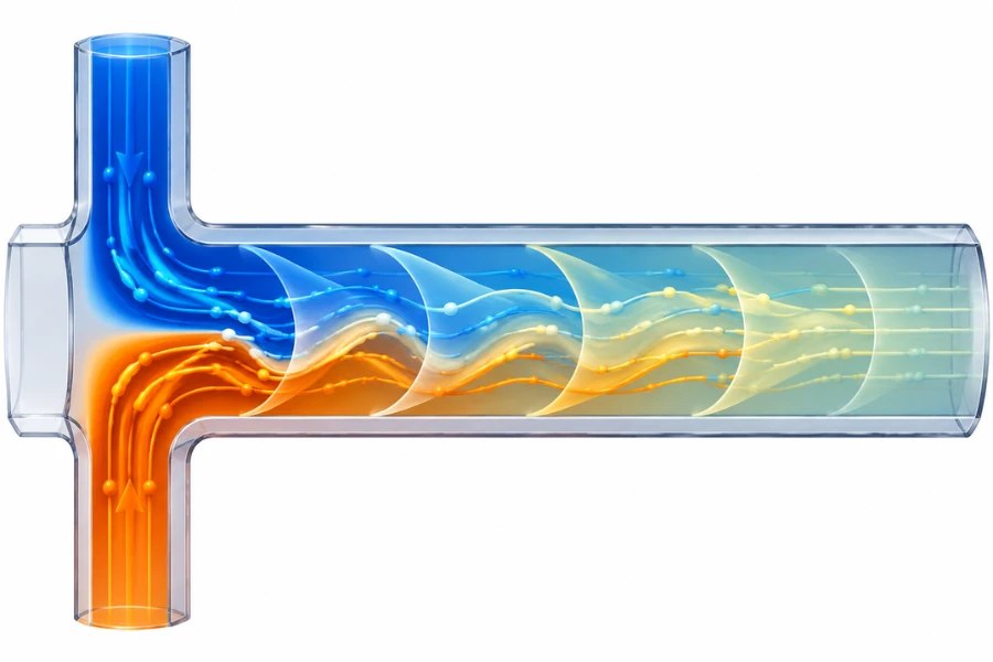
Mixing Time Distribution (MTD) provides a more detailed representation of this variation.

A Lagrangian particle-tracking workflow can identify the mixing times of individual fluid elements.

1. Calculate velocity and concentration fields using a validated CFD model.
2. Release representative virtual particles from defined inlet positions.
3. Track their trajectories through the mixing structure.
4. Evaluate concentration variation along each trajectory.
5. Determine when each trajectory reaches the specified mixing criterion.
6. Compare the resulting distribution across operating conditions.

The mixing endpoint must be defined explicitly. A study may use a concentration tolerance or a specified mixing-intensity threshold.

A 2026 study by Liu and coauthors applied a Lagrangian framework to MTD in T-shaped microreactors, using particle trajectories extracted from CFD simulations to map differences in individual mixing histories.

Mixing Surface Tracking (MS-T) is related but distinct. It evaluates the evolution of surfaces formed by fluid elements with equal mixing times rather than reporting only the distribution of individual mixing times.

A separate 2026 study by Liu and coauthors used a reaction-free CFD framework to examine mixing surfaces and mixing intensity. Its selected threshold of 0.95 was a study-specific endpoint criterion, not a universal requirement.

These approaches are particularly useful when reaction performance is sensitive to local mixing histories rather than only average homogenization time.

Mixing Time vs. Reaction Time

The mixing-to-reaction time ratio helps identify whether a process may be mixing-limited.

\frac{t_{\mathrm{mix}}}{t_{\mathrm{reaction}}}]

This article uses (\Psi_{\mathrm{mix}}) as a defined mixing-to-reaction timescale ratio, not as a universal Damköhler number convention.

• If (\Psi_{\mathrm{mix}}\ll1), mixing is generally faster than the characteristic reaction process.
• If (\Psi_{\mathrm{mix}}) approaches 1, mixing and reaction occur on comparable timescales.
• If (\Psi_{\mathrm{mix}}\gg1), reaction may proceed before sufficient homogenization occurs.

The actual effect depends on reaction order, competing pathways, local concentration fields, and the definition of characteristic reaction time.

How Mixing and RTD Affect Chemical Reaction Performance

Mixing and RTD influence reaction performance through different mechanisms. Their relative importance depends on reaction kinetics, heat release, phase behavior, and the sensitivity of product properties to local conditions.

Local Concentration Gradients and Selectivity

In competing reaction pathways, local concentrations influence relative reaction rates.

A rapidly reacting feed introduced into a poorly mixed stream can create a region with high local reactant concentration. This may favor a secondary reaction even when the average reactor composition is suitable.

Micromixers reduce these differences by shortening diffusion distances or redistributing fluid streams. However, improved mixing alone cannot eliminate variability caused by RTD, temperature gradients, catalyst activity, or feed composition.

حدود انتقال الحرارة والكتلة

High surface-area-to-volume ratios can improve heat transfer, but they do not guarantee that heat removal keeps pace with reaction heat release.

For strongly exothermic reactions, engineers should compare reaction timescales with heat and mass transfer timescales. Relevant variables include heat-release rate, thermal properties, wall temperature, channel dimensions, heat-transfer resistance, and operating pressure.

Mixing, reaction kinetics, and heat removal must therefore be evaluated together when defining operating limits.

Multiphase Reaction Considerations

Gas-liquid and liquid-liquid microreactors introduce interfacial transport mechanisms that can influence mixing and RTD.

In liquid-liquid systems, droplet size, phase ratio, interfacial area, and flow pattern affect mass transfer. In gas-liquid systems, bubble velocity, gas holdup, and interfacial renewal influence contact time and transport rates.

A single-phase axial dispersion model may not adequately represent these systems. RTD measurements should be accompanied by flow-pattern observation, phase distribution measurements, and mass-transfer evaluation where appropriate.

Reaction Type	Potential Limitation	Important Evaluation Parameters
Fast competitive reactions	Local concentration gradients	Mixing time and DOM
Highly exothermic reactions	Local temperature differences	Heat transfer and temperature distribution
Precipitation	Local supersaturation differences	Mixing history and nucleation conditions
البلمرة	Different reaction histories	RTD and mixing-time distribution
Multiphase reactions	Insufficient interfacial transport	Interfacial area and mass-transfer coefficient

Microreactor Scale-Up Methods and Design Equations

Microreactor scale-up must increase production capacity without losing the transport characteristics responsible for laboratory-scale performance.

The two principal approaches are numbering-up and sizing-up. Hybrid strategies combine both.

Numbering-Up and Parallel Channel Design

Numbering-up increases production capacity by connecting multiple similar reaction channels or reactor units in parallel.

For (N) identical circular channels:

N\frac{\pi D^2L}{4}]

Where (D) is channel diameter and (L) is channel length.

Under uniform flow distribution:

\frac{Q_{\mathrm{total}}}{N}]

This assumes identical geometry and hydraulic conditions.

In practice, manufacturing tolerances, manifold geometry, pressure differences, viscosity variations, and partial blockages can produce unequal flow rates.

For channels with identical internal volumes:

[\tau_i=\frac{V_i}{Q_i}]

A channel receiving a higher flow rate has a shorter nominal residence time, potentially producing differences in conversion and selectivity across the reactor assembly.

Numbering-up therefore requires a flow distribution system capable of maintaining consistent hydraulic conditions, not merely an increase in channel count.

Sizing-Up and Geometric Similarity

Sizing-up increases capacity by modifying individual channel dimensions, length, or both.

For a circular channel, the internal surface-area-to-volume ratio is:

[\frac{A_s}{V}=\frac{4}{D}]

Increasing diameter reduces this ratio and increases transverse diffusion distance. Pressure drop, velocity distribution, and flow regime may also change.

Simply increasing channel diameter while maintaining nominal residence time does not guarantee equivalent reactor performance.

A sizing-up strategy should identify which performance criteria must remain comparable, including mixing time, RTD, heat-transfer performance, mass-transfer coefficient, pressure drop, and energy dissipation.

Energy Dissipation-Based Scale-Up

For mixing-intensive liquid-liquid systems, average energy dissipation rate can provide an additional scale-up criterion.

[\varepsilon=
\frac{\Delta P Q}{\rho V}]

Where (\varepsilon) is average energy dissipation rate per unit mass, (\Delta P) is reactor pressure drop, (Q) is volumetric flow rate, (\rho) is fluid density, and (V) is the relevant reactor volume.

This relationship assumes that hydraulic power loss is dissipated within the defined control volume. Pressure losses in pumps, connecting lines, and external components should be separated from reactor pressure drop.

Plouffe and coauthors investigated sizing-up for liquid-liquid microreactors using a 3/7 scaling rule. Their 2016 study compared mixers with hydraulic diameters of approximately 283 μm and 714 μm.

At the designed operating conditions, the larger mixer operated at flow rates approximately 8.5 times higher while maintaining comparable average energy dissipation. Similar overall volumetric mass-transfer coefficients were reported at equivalent energy dissipation rates within the investigated drop-flow regime.

This is an experimental example, not a universal scaling law. Its applicability depends on geometry, phase behavior, flow regime, and fluid properties.

Hydrodynamic Similarity During Scale-Up

Geometric similarity does not automatically produce hydrodynamic similarity. Two reactors with similar shapes may have different Reynolds numbers, Péclet numbers, pressure drops, and mixing times.

المعلمة	What It Represents	Scale-Up Consideration
Reynolds Number	Inertial-to-viscous force ratio	Flow regime and secondary flow
Péclet Number	Convective-to-diffusive transport ratio	Mixing and dispersion
Schmidt Number	Momentum-to-mass diffusivity ratio	Fluid transport properties
Damköhler Number	Reaction-to-transport relationship	Reaction limitations
انخفاض الضغط	Hydraulic resistance	Pumping requirements
Energy Dissipation	Mechanical energy input per unit mass	Mixing-intensive processes

The relevant criteria should be selected according to reaction mechanism and reactor configuration. Preserving one dimensionless number does not necessarily preserve every transport characteristic.

Hybrid Scale-Up Strategies

A hybrid strategy combines moderate increases in individual channel dimensions with parallelization.

An engineering team may first increase the capacity of an individual reactor module while maintaining acceptable mixing and heat-transfer characteristics. Additional modules can then be connected in parallel to achieve the required production rate.

This approach can reduce the manifold complexity of extremely large numbering-up systems while retaining modularity.

Each scale-up stage still requires validation of pressure distribution, flow uniformity, residence time, and reaction performance.

DODGEN’s microchannel reaction technology provides an industrial context for integrating controlled reactant distribution, engineered mixing structures, and modular reactor configurations.

Maintaining RTD Consistency in Industrial Microreactor Systems

Industrial numbering-up introduces a distinction between individual channel performance and overall reactor performance. A parallel assembly can meet its total flow target while individual channels operate under different hydraulic conditions.

Flow Maldistribution in Parallel Channels

Flow maldistribution occurs when parallel channels receive unequal volumetric flow rates.

Contributing factors include differences in channel diameter or length, asymmetric manifolds, unequal inlet and outlet pressure, fabrication tolerances, deposits, partial blockages, and changes in fluid viscosity.

The relative sample standard deviation of channel flow rates can be calculated as:

[CV_Q=
\frac{1}{\bar Q}
\sqrt{
\frac{1}{N-1}
\sum_{i=1}^{N}(Q_i-\bar Q)^2
}
\times100%]

Where (Q_i) is the flow rate in channel (i), (\bar Q) is average channel flow rate, and (N) is the number of channels.

A lower CV indicates more uniform distribution. Acceptable limits should be established according to reaction sensitivity and product specifications rather than assuming a universal tolerance.

Engineering Calculation Example for Flow Maldistribution

Consider a parallel reactor system with 25 channels. Each channel has an internal volume of 1 mL, and the total system flow rate is 25 mL/min.

Under ideal conditions:

[Q_i=\frac{25}{25}=1\ \mathrm{mL/min}]

The nominal residence time in each channel is:

[\tau_i=\frac{1}{1}=60\ \mathrm{s}]

Now assume four channels experience different flow rates, while the remaining 21 channels continue operating at 1 mL/min.

Channel	Flow Rate (mL/min)	Nominal Residence Time (s)
1	0.90	66.67
2	0.95	63.16
3	1.00	60.00
4	1.05	57.14
5	1.10	54.55
6–25	1.00	60.00

The total flow remains:

[Q_{\mathrm{total}}=25\ \mathrm{mL/min}]

The sample flow coefficient of variation is:

[CV_Q\approx3.23%]

The flow-weighted mean residence time remains 60 seconds because the channel volumes are identical and total flow is unchanged.

The between-channel contribution to RTD variance is:

\sum_iw_i(\bar t_i-\bar t_{\mathrm{system}})^2]

المكان:

[w_i=\frac{Q_i}{Q_{\mathrm{total}}}]

Using the assumed flow rates:

[\sigma_{\mathrm{between}}^2
\approx3.631\ \mathrm{s}^2]

لذلك:

[\sigma_{\mathrm{between}}\approx1.91\ \mathrm{s}]

This value represents differences between channel mean residence times. It excludes additional axial dispersion within individual channels.

The calculation demonstrates why an acceptable overall flow rate does not establish uniform processing conditions across a parallel reactor assembly.

Manifold and Flow Distributor Design

Flow distributors should deliver sufficiently uniform pressure and flow conditions across parallel channels.

Important design variables include inlet and outlet symmetry, distribution-channel dimensions, branch hydraulic resistance, distributor pressure loss, flow separation, and cleaning access.

An effective distributor balances flow uniformity with energy consumption and pressure drop. Excessive hydraulic resistance may improve flow balancing but increase pumping requirements.

Hydraulic Resistance and Pressure Drop

For fully developed laminar flow in a straight circular tube, the Hagen-Poiseuille equation gives:

[\Delta P=
\frac{8\mu LQ}{\pi R^4}]

Where (\mu) is dynamic viscosity, (L) is channel length, (Q) is volumetric flow rate, and (R) is internal radius.

The fourth-power dependence on radius makes hydraulic resistance sensitive to channel dimensions. Small fabrication deviations can therefore produce differences in pressure drop and flow distribution.

For a simplified laminar flow network:

[\Delta P=R_hQ]

Where (R_h) is hydraulic resistance.

This relationship supports parallel branch analysis, with flow through each channel determined by its pressure difference and hydraulic resistance.

The Hagen-Poiseuille equation applies to fully developed laminar flow in circular tubes. Rectangular and other noncircular channels require geometry-specific relationships.

CFD Modeling and Experimental Validation

CFD can identify velocity fields, pressure distribution, flow separation, and manifold performance before equipment fabrication.

For single-phase, low-Reynolds-number applications, simulations commonly begin with incompressible laminar flow assumptions. More complex systems may require multiphase interfaces, heat transfer, species transport, reaction kinetics, non-Newtonian rheology, and surface interactions.

Model credibility depends on mesh quality, boundary conditions, accurate fluid properties, numerical convergence, and experimental validation.

In convection-dominated channels, numerical diffusion can artificially broaden concentration profiles and overpredict mixing. Mesh sensitivity and species transport discretization should therefore be evaluated before interpreting simulated mixing indices or RTD predictions.

A practical workflow includes:

1. Establish realistic geometry and fluid properties.
2. Define inlet, outlet, and wall boundary conditions.
3. Verify mesh independence and numerical convergence.
4. Calculate velocity, pressure, and species concentration fields.
5. Track fluid elements when residence time or mixing history is required.
6. Compare predicted pressure drop, RTD, or mixing indices with experimental measurements.

A combined approach using CFD, simplified hydraulic network models, and targeted experiments can provide the information required for full-system design without relying exclusively on computational simulation.

RTD Consistency Across Parallel Reactor Channels

The measured RTD of a complete parallel assembly may conceal differences between individual channels.

For an idealized set of parallel channels receiving a uniform tracer input, the overall RTD is a flow-weighted combination of the individual channel distributions.

\sum_{i=1}^{N}
\frac{Q_i}{Q_{\mathrm{total}}}E_i(t)]

Where (E_i(t)) is the RTD of channel (i).

The overall variance contains contributions from both within-channel dispersion and differences between channel mean residence times.

\sum_iw_i
\left[
\sigma_i^2+
(\bar t_i-\bar t_{\mathrm{system}})^2
\right]
]

المكان:

[w_i=\frac{Q_i}{Q_{\mathrm{total}}}]

Improving individual channel hydrodynamics addresses within-channel dispersion. Improving manifold design and flow distribution addresses between-channel variation.

Both mechanisms must be evaluated during industrial numbering-up.

Fouling and Long-Term RTD Stability

Deposits, polymer buildup, precipitation, and other forms of fouling can reduce effective channel diameter during extended operation.

For laminar flow in a circular channel, a reduction in radius increases hydraulic resistance substantially because of its fourth-power dependence. Uneven fouling across parallel channels can redirect flow toward less restricted branches and change individual residence times.

A monitoring strategy should therefore consider differential pressure, total flow rate, feed properties, cleaning frequency, and periodic tracer-based RTD verification.

Processes prone to deposition or blockage also require inspection access, cleaning procedures, and defined operating limits.

From Pilot Validation to Commercial Microreactor Deployment

Commercial deployment requires more than demonstrating that a reaction works in a laboratory microchannel. The integrated process must maintain acceptable hydrodynamic, thermal, and chemical performance under realistic operating conditions.

Laboratory Hydrodynamic Characterization

The laboratory reactor establishes the reference performance for scale-up.

Relevant measurements include mean residence time, RTD variance, axial dispersion coefficient, mixing time, degree of mixing, pressure drop, heat-transfer behavior, and flow distribution.

Testing should use representative fluid properties and operating conditions. Water-based measurements alone may not represent a process using fluids with substantially different viscosities, diffusivities, or phase behavior.

Model Calibration and Pilot-Scale Validation

Experimental data should be used to calibrate the selected hydraulic and dispersion models.

For numbering-up, pilot validation should focus on channel-to-channel flow uniformity. For sizing-up, engineers should evaluate whether mixing, RTD, heat transfer, and mass transfer remain acceptable at the larger dimensions.

Pilot testing should demonstrate repeatable operation, stable flow distribution, acceptable pressure drop, and consistent product quality over a representative operating period.

Pilot-Scale Performance Acceptance

Laboratory and pilot configurations should be compared under equivalent and documented process conditions.

Validation Parameter	What to Evaluate	Engineering Purpose
Mean Residence Time	Difference between measured values	Confirm contact-time consistency
Normalized RTD Variance	Distribution width	Identify additional dispersion
Mixing Time	Time to reach selected mixing criterion	Evaluate micromixing
Degree of Mixing	Cross-sectional concentration uniformity	Compare mixing quality
انخفاض الضغط	Reactor and distributor losses	Verify hydraulic feasibility
Conversion and Selectivity	Product performance	Confirm reaction consistency
Long-Term Flow Stability	Changes during extended operation	Assess operating reliability

Acceptance limits should reflect reaction kinetics, product specifications, measurement uncertainty, and equipment limitations. A fast competitive reaction may require tighter mixing and RTD control than a slower reaction with broader operating tolerances.

Continuous Production Stability

Extended operation introduces conditions that may not appear during short laboratory tests. These include fouling, progressive pressure-drop changes, feedstock variability, pump fluctuations, thermal drift, and startup and shutdown transients.

Pressure-drop trends can provide an early indication of channel restriction. Changes in feed composition or viscosity may also require adjustments to flow settings or temperature control.

The control strategy should define monitoring parameters and operating limits that maintain reproducible process conditions throughout the production cycle.

Process Integration and Commercial Feasibility

Microreactors are often part of a larger continuous manufacturing system that includes feed preparation, heat exchange, reaction control, separation, purification, solvent recovery, and downstream product handling.

These operations must be evaluated together because upstream and downstream equipment can influence reactor operating conditions.

A technically successful microreactor is not necessarily commercially viable if the integrated system cannot meet throughput, reliability, energy, maintenance, and product-quality requirements.

DODGEN’s continuous flow reactor solutions cover related equipment categories, including microreactors, static mixers, polymerization reactors, and heat exchangers. Its حلول تكنولوجيا العمليات provide a broader context for process development, pilot testing, and integration.

Scale-up should therefore be treated as a process engineering task rather than a simple increase in reactor volume or channel count.

الخاتمة

Microreactor design requires separate but coordinated evaluation of mixing and residence time distribution. Mixing-time correlations quantify homogenization, while tracer-based RTD measurements and axial dispersion models characterize the residence time history of fluid elements.

During scale-up, preserving individual channel performance is only part of the challenge. Flow distribution, manifold resistance, pressure drop, fouling, and long-term operating stability determine whether the integrated system can maintain consistent production.

الأسئلة الشائعة